RNA-seq / Differential expression using edgeR for multivariate experiments
Description
Differential expression analysis for multifactor experiments using the generalized linear models (glm) -based
statistical methods of the edgeR Bioconductor package.
Parameters
- Main effect 1
- Main effect 2
- Main effect 3
- Treat main effect 1 as factor (yes, no) [yes]
- Treat main effect 2 as factor (yes, no) [yes]
- Treat main effect 3 as factor (yes, no) [yes]
- Include interactions in the model (yes, no, nested) [no]
- Apply TMM normalization (yes, no) [yes]
- Filter out genes which don't have counts in at least this many samples (1-10000) [1]
- Plot width (200-3200 [600]
- Plot height (200-3200) [600]
- Give as an output the design matrix (yes, no) [no]
Details
This tool takes as input a table of raw counts from the different samples. The count file has to be associated
with a phenodata file describing the experimental factors.
You can generate these files using the
Define NGS experiment
tool, which combines count files for different samples to one table and creates a phenodata file for it.
We recommend marking the control group with 0 and the other groups with 1,2,3... in the phenodata
columns.
The group with the smaller number (or, if using letters, the alphabetically first letter) is used as the
baseline.
This means that in the results table, positive fold changes are upregulated and negative downregulated
genes compared to the control group.
You should set the filtering parameter to the number of samples in your smallest experimental group.
Filtering will cause those genes which are not expressed or are expressed in very low levels (less than 5
counts) to be ignored in statistical testing.
These genes have little chance of showing significant evidence for differential expression, and removing them
reduces the severity of multiple testing correction of p-values.
Trimmed mean of M-values (TMM) normalization is used to calculate normalization factors in order to reduce RNA
composition effect,
which can arise for example when a small number of genes are very highly expressed in one experiment condition
but not in the other.
Dispersion is estimated using Cox-Reid profile-adjusted likelyhood (CR) method. Trended dispersions are
estimated prior to estimating tagwise dispersions.
After dispersion estimation, negative binomial generalized linear models are fitted to the data,
after which the differentially expressed genes are determined using quasi-likelihood (QL) F-test.
You can read more about these methods in the edgeR user guide linked below.
Statistical analysis to identify differentially expressed genomic features (genes, miRNAs,...) is performed
using a multivariate regression model. A maximum of three different variables, and their interactions
can be specified for the model. It is highly recommended to always have at least two biological replicates for
each experiment condition.
Note, that unlike with basic edgeR or DESeq2, no filtering is done to the results table.
Please notice that in the results table you will have all the comparisons between the different effects defined
in the parameters -section.
You can filter the table for example based on the adjusted p-values (FDR-columns) using the tool
Utilities /
Filter table by column value .
Choosing the effects and understanding the results
What are then the questions you want to ask, what are the comparisons you want to make?
We recommend reading
Chapter 3.2.4 "Questions and Contrasts" in edgeR user guide for a nice overview.
EdgeR's glm mode used in this tool uses a design matrix to determine the sample groups and
creates the contrasts based on those.
In Chipster, this design matrix is generated from the phenodata file based on the parameters you choose
(Main effects 1-3 and how to treat the interaction terms).
The contrasts (comparisons) are always done and reported in the result table in the same way in Chipster.
The same statistics (listed below in the Output section) columns are reported for all the comparisons.
If you wish to see what the design matrix looks like, you can ask the tool to give it as an output.
The first columns in the table, marked "Intercept", are measuring the baseline in the first treatment
condition, and the comparisons after that are relative to this baseline.
This makes sense, when the first condition ("group") is the control group.
This assumption means, that Chipster doesn't automatically allow you to create all the different comparisons:
for example, if you have 3 groups, A, B and C, Chipster can only give you the comparisons A vs B and A vs C
(A is considered as the "control" here).
To get the third comparison (B vs C), you need to run the tool again and change the order of the groups,
so that for example B = control (= marked with the lowest number in the phenodata file). As a result
from this comparison you would get: B vs A (which you already had, just the other way around) and B vs C.
In the result table, you can see which comparison is in question from the column name:
for example, Pvalue(group)2 is the (unadjusted) p-value for the comparison between the first (=control,
baseline)
and the second groups in the "group" column.
Which effects should I include in the model? You can estimate this from looking at the PCA plot
(try the tool PCA and heatmap of samples with
DESeq2).
If you can see some of the effects there, it is advisable to add them to the model.
Adding the batch effects to the model corrects for them, and your comparison of the actual groups of
interest will be clearer. This effect is demonstrated in the example session
course_RNAseq_parathyroid_done,
where you are not able to find any differentially expressed genes before you add all the relevant effects to the
model.
Including interactions
You can choose whether you want to include only the main effects ("Include interactions in the model" = "no"),
the main effects and all the interaction terms ("yes"), or
the main effect 1 and its interactions with main effects 2 and 3 ("nested", see more information about this
option below).
As a rule of thumb, you can add the interactions when you think they are relevant.
Paired samples: for paired samples, do not include the interaction terms. See
Chapter 3.4.1 "Paired samples" in edgeR user guide for more information.
Example of the use of the "nested" option:
The "nested" option is needed when you want to do comparisons both between and within subjects
(you might want to see the chapter 3.5. in
EdgeR userguide.
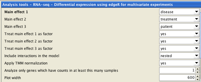
If you are using "nested" option, note that you need to choose the effects accordingly:
Main effect 1 = the group in which the comparison is done between the subjects ("disease" in the example)
Main effect 2 = the group in which the comparison is done within the subjects ("treatment" in the example)
Main effect 3 = the subjects / column explaining the pairing of the samples ("patient" in the example)
We have an experiment with 3 cancer patients and 3 controls. There are 2 samples from each patient, before and
after the treatment.
The normal-cancer comparison is thus done between individuals, while the untreated-treated comparison is done
within individuals.
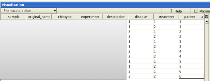
In the phenodata-file we mark create corresponding groups:
disease = normal/cancer
treatment = untreated/treated
patient = the individuals
Note that you want to mark the "control"-situation (normal patient, untreated) with smaller index.
In the parameters-section, we choose the "nested" -option and the effects:
In the resulting edger_glm.tsv -file there will be several columns corresponding to the different comparisons.
In
the example situation:
as.factor(disease) = comparison between the cancer patients and the controls
as.factor(disease)1:as.factor(treatment)2 = comparison between the untreated and treated control patients
as.factor(disease)2:as.factor(treatment)2 = comparison between the untreated and treated cancer patients
Output
- edger_glm.tsv: Table containing the statistical testing results, including fold change and p-values.
- logFC = log2 fold change between the groups. E.g. value 2 means that the expression has increased 4-fold
- logCPM = the average log2-counts-per-million
- LR = likelihood ratio statistics
- PValue = the two-sided p-value
- FDR = adjusted p-value
- dispersion-edger-glm.pdf: Biological coefficient of variation plot.
- design-matrix.tsv: the design matrix created based on the phenodata file and parameter selections (optional
output).
References
This tool uses the edgeR package for statistical analysis. Please cite the following articles:
MD Robinson, DJ McCarthy and GK Smyth.
edgeR: a Bioconductor package for differential expression analysis of digital gene expression data.
Bioinformatics, 26 (1):139-40, Jan 2010.
DJ McCarthy, Y Chen and GK Smyth.
Differential expression analysis of multifactor RNA-Seq experiments with respect to biological variation.
Nucleic Acids Res, 40 (10):4288-97, May 2012.
More information about the functions can be found also in the
EdgeR Users Guide